
The Loudness Analyzer & Normalizer is a tool that is useful at the end of the mixing process to make the final audio file comply with different specs regarding loudness.
It is enabled by checking “Enable Master-Bus Output Gain Control” in the Preferences:
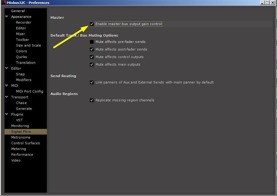
The Master Bus strip then shows a button marked “LAN”, and a volume slider that is the global gain that can be set either manually or by the loudness normalizer.
The LAN can also be started from “Session -> Loudness Assistant”. If the option above is not enabled, Mixbus will open the relevant page of the Preferences.
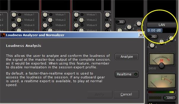
Click on “Analyze” to start the loudness analysis. A choice is offered between freewheeling (i.e. Mixbus renders the session as fast as possible to measure the loudness) by default, or Realtime, for cases where freewheeling would not accurately render the session. This might be the case if a hardware or JACK effect is used in the session.
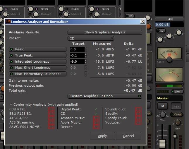
After the analysis is over, the Loudness Analyzer and Normalizer is shown:
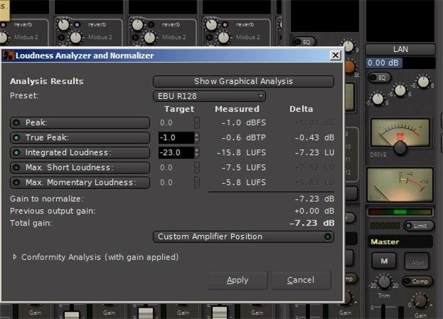
A number of different statistics are displayed for the standard indicated in the “PRESET” tab. The analysis standard can be changed with the “PRESET” tab:
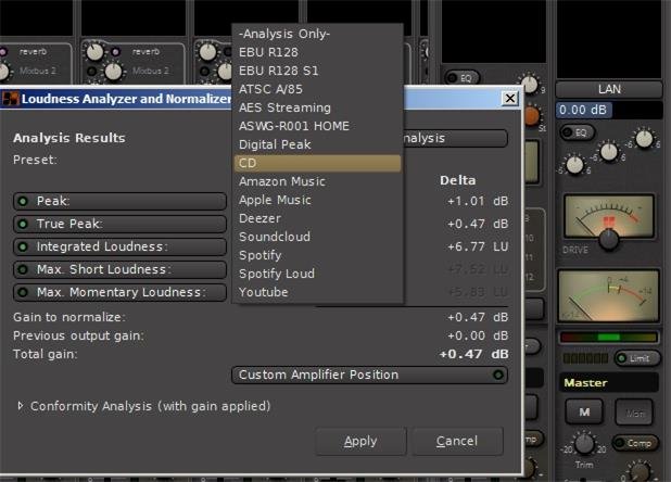
Notice in the next figure that a different set of analysis statistics will be presented.
Normalization Parameters
As loudness is a perceived sonic energy, and depends on the level, frequency, duration and nature of the sound, this window allows to base the calculation of the loudness normalization on different parameters :
Peak : is the highest signal level value
True Peak : is the highest signal level value where the signal has been oversampled to figure out more in-between values between the samples (interpolation)
Integrated Loudness : is the loudness computed from the whole session or range
Max Short Loudness : is the maximum loudness computed on short time ranges (3 seconds)
Max Momentary Loudness : is the maximum momentary loudness
Any combination of these parameters can be taken into account when determining the gain normalization, by checking its momentary button, and setting a Target value.
Shown are both the Measured value of the parameters, and the Delta value, i.e. the difference between the Target and Measured values, hence the gain correction. The maximum Delta value is the Gain correction to apply to fit all the Target values.
Also shown under the parameters is a summary of the calculation :
Gain to Normalize: is the max Delta value
Previous Output Gain: is the current Master track gain
Total Gain: is the difference between these two values, hence the correction to apply
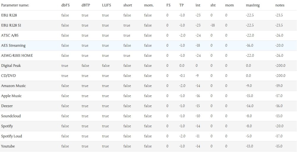
Presets
A selection of presets is offered to simplify the normalization. These presets apply the relevant parameters and their target values. Here is a table of these presets:
The Conformity Analysis Panel
At the bottom of the window the Conformity Analysis arrow can be rotated to display, for the presets above, if the corrected gain would fit the required values:
✖: the signal is too loud
✔: the signal is too quiet, but satisfies the max. loudness spec
✔: signal loudness is within the spec.
Notice here as we have run the analysis for only the CD case, only the digital peak (applicable to ALL formats) and the CD case are checked.
Lastly, the gain correction is, by default, applied after all the processors of the master bus. This can also be changed, either by selecting the Custom Amplifier Position button in this window, or in the Master strip, by Right-clicking the gain slider and selecting the Custom LAN Amp Position. The gain normalizer then becomes a processor in the processors box of the Master strip, that can be moved as needed like any processor/effect:
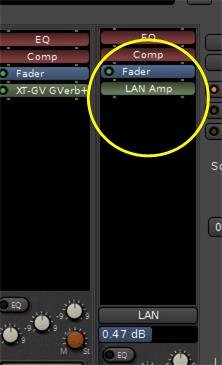
Notice here that with the gain normalizer added, +0.47 dB of gain (as was indicated in the last figure) has been added as a result of the normalization.
To show the results graphically, click on the “Show Graphical Analysis” button:
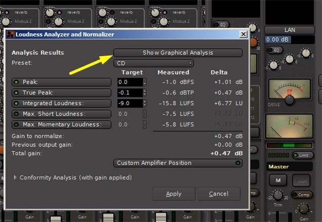
A graphical representation of the analysis will be displayed:
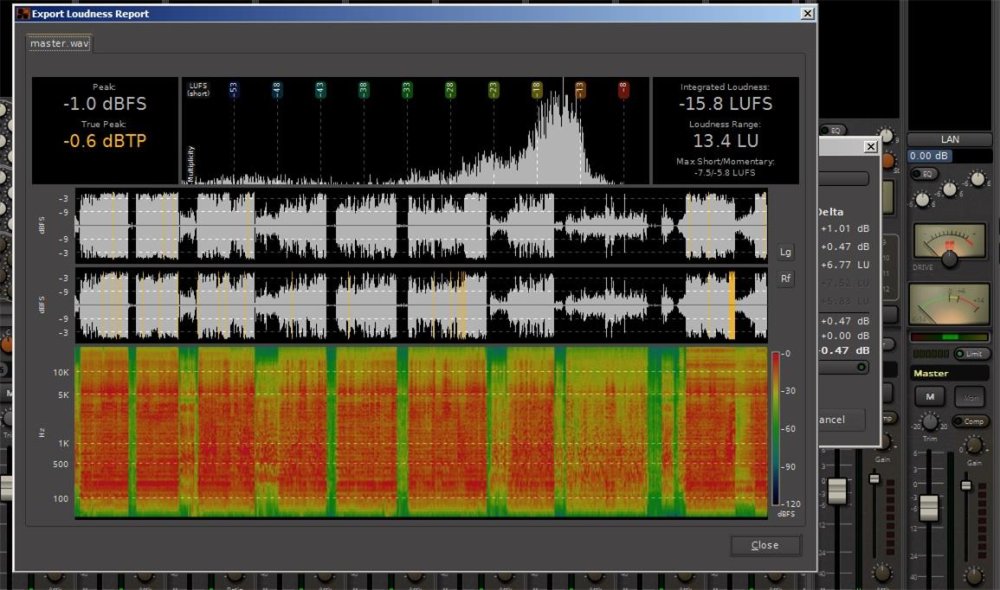
At the top of the graphical analysis is a histogram of the levels in the recording, i.e. how often (vertical axis) the signal spends at various levels (horizontal axis). In this example we see that the signal is between -33 and -8 dBFS most of the time.
In the middle are the Left and Right output waveforms. The coloured vertical bars in the waveform indicate where the signal is at True Peak shown in the histogram statistic above.
At the bottom is a frequency distribution histogram with time (horizontal axis) and frequency (vertical axis). This histogram indicates by colour (legend to the right) the levels of the frequencies present in the signal versus time.
Post your comment on this topic.